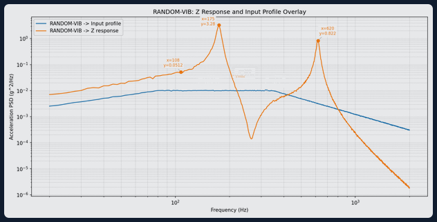
Show the input. Otherwise the peak can mislead.
Quick answer
Plot the response and the measured input against the same frequency axis, with compatible units and clear labels. Mark response peaks using documented selection rules. Show the requested input target separately from the measured input so a controller deviation is not mistaken for structural behaviour.
Method
Identify whether each curve is sine amplitude, PSD, ASD or a transfer quantity. Confirm acceleration units and whether amplitudes are peak or RMS.
Select a response channel and its corresponding excitation/control channel from the same run. Retain channel identities and acquisition settings.
Plot on a shared frequency axis. Use log axes only for positive values. Do not silently remove zero or invalid samples; document exclusions.
For matching quantities and units, use the same vertical scale. If units differ, prefer aligned separate panels over a misleading overlay. Do not put a PSD and sine amplitude on one common acceleration scale.
Add the target profile as a distinct line, labelled target. Label the measured input explicitly, including any control aggregation such as an average of sensors.
Detect local maxima within a stated frequency band, using a chosen minimum separation. Mark only defensible peaks with frequency, amplitude and units. Retain enough information to reproduce selection.
Review peaks against input features, notches and noise. If analysing a transfer response, create a separately labelled response/input plot and document how it was formed.
Limitations
A visible maximum can reflect excitation shape, not a mode. Coarse spacing and smoothing can move or merge peaks. A marked peak does not establish Q, damping or a qualification limit. Never label a target curve as measured input. Export with readable axes, legend, channel names and method notes.
How TDC helps
TDC accepts CSV, TSV, XLS, XLSX, UNV and UFF vibration test files. It plots the response and the input_profile channel on one shared axes and marks the top peaks (default 3) on the response. Random-vibration plots start at 20 Hz unless a lower bound is set; log axes are available. Values are computed in code from measured data, not invented by AI.
Request access to TDC at https://oxorigin.com/products/tdc or contact@oxorigin.com.
Example
Simulated random vibration response PSD with input profile from 20 to 2000 Hz (measurement RANDOM-VIB).
"Plot Z response and the input profile from measurement RANDOM-VIB, on the same graph, and mark the top 3 peaks on the response"